C/1946 C1 Timmers
more info
Comet C/1946 C1 was discovered on 2 February 1946 by Matthew Timmers (Vatican Observatory, Castel Gandolfo, Italy). Soon, a few prediscovery images (23, 24, 28 and 29 of January), were found by Fred L. Whipple. At the moment of discovery, the comet was over two months before perihelion passage, and it was last seen on 9 August 1947. [Kronk, Cometography: Volume 4].
This comet made its closest approach to the Earth on 6 February 1946 (1.016 au), that is four days after its discovery.
Solutions given here was based on data spanning over 1.526 yr in a range of heliocentric distances from 1.973 au through perihelion (1.724 au) to 5.559 au.
Pure gravitational orbit determined from the available positional measurements (485 observations) give 1a-class orbit.
It was possible to determine the non-gravitational orbit for C/1946 C1 (preferred orbit) where a noticeable decrease of RMS was obtained (from 2.54 arcsec to 2.17 arcsec, see below) and some trends in right ascension and declination were reduced (see figure). This NG-solution give more tight original orbit than pure gravitational solution.
This probably Oort spike comet suffers moderate planetary perturbations during its passage through the planetary system that lead to a more tight future orbit with semimajor axis less than 3000 au (see future barycentric orbits for both models of motion).
More details in Królikowska et al. 2014.
| solution description | ||
|---|---|---|
| number of observations | 485 | |
| data interval | 1946 01 29 – 1947 08 09 | |
| data type | perihelion within the observation arc (FULL) | |
| data arc selection | entire data set (STD) | |
| range of heliocentric distances | 1.97 au – 1.72 au (perihelion) – 5.56 au | |
| type of model of motion | NS - non-gravitational orbits for standard g(r) | |
| data weighting | YES | |
| number of residuals | 848 | |
| RMS [arcseconds] | 2.17 | |
| orbit quality class | 1b | |
| next orbit statistics, both Galactic and stellar perturbations were taken into account | ||
|---|---|---|
| no. of returning VCs in the swarm | 5001 | * |
| no. of escaping VCs in the swarm | 0 | |
| no. of hyperbolas among escaping VCs in the swarm | 0 | |
| next reciprocal semi-major axis [10-6 au-1] | 339.69 – 346.97 – 354.15 | |
| next perihelion distance [au] | 1.72051 – 1.72054 – 1.72057 | |
| next aphelion distance [103 au] | 5.65 – 5.76 – 5.89 | |
| time interval to next perihelion [Myr] | 0.15 – 0.154 – 0.159 | |
| percentage of VCs with qnext < 10 | 100 | |
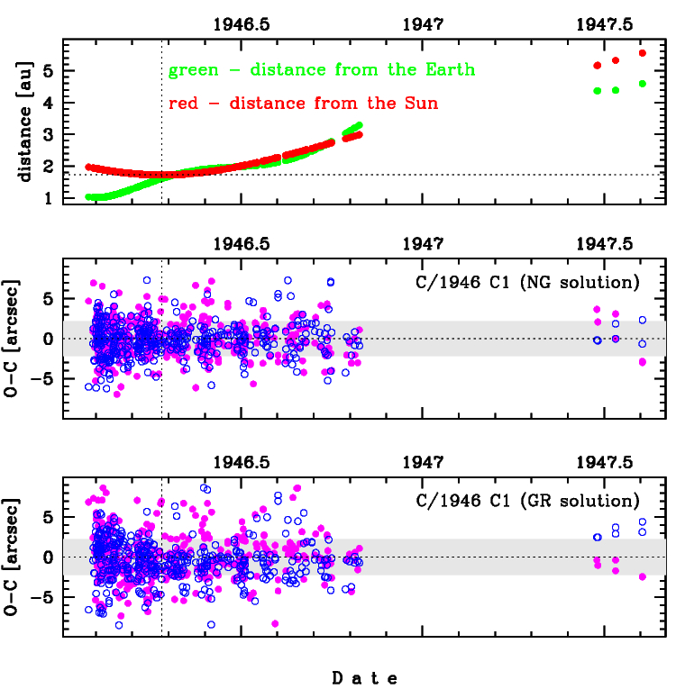
Upper panel: Time distribution of positional observations with corresponding heliocentric (red curve) and geocentric (green curve) distance at which they were taken. The horizontal dotted line shows the perihelion distance for a given comet whereas vertical dotted line — the moment of perihelion passage.
Lower panel (panels): O-C diagram for this(two) solution (solutions) given in this database, where residuals in right ascension are shown using magenta dots and in declination by blue open circles.
Lower panel (panels): O-C diagram for this(two) solution (solutions) given in this database, where residuals in right ascension are shown using magenta dots and in declination by blue open circles.
| next_g orbit statistics, here only the Galactic tide has been included | ||
|---|---|---|
| no. of returning VCs in the swarm | 5001 | * |
| no. of escaping VCs in the swarm | 0 | |
| no. of hyperbolas among escaping VCs in the swarm | 0 | |
| next reciprocal semi-major axis [10-6 au-1] | 339.69 – 346.97 – 354.15 | |
| next perihelion distance [au] | 1.72019 – 1.7202 – 1.7202 | |
| next aphelion distance [103 au] | 5.65 – 5.76 – 5.89 | |
| time interval to next perihelion [Myr] | 0.15 – 0.154 – 0.159 | |
| percentage of VCs with qnext < 10 | 100 | |