C/1959 Y1 Burnham
more info
Comet C/1959 Y1 was discovered on 30 December 1959 by Robert Burnham Jr (Lowell Observatory, Arizona, USA), that is 5 months before its perihelion passage. It was observed until 13 July 1960 [Kronk, Cometography: Volume 4].
Comet had its closest approach to the Earth on 27 April 1960 (0.203 au), 12 days after its perihelion passage.
This is a comet with nongravitational effects strongly manifested in positional data fitting.
Both solutions (GR and NG) given here are based on data spanning over 0.449 yr in a range of heliocentric distances: 1.63 au – 0.504 au (perihelion) – 1.81 au.
This Oort spike comet suffers moderate planetary perturbations during its passage through the planetary system; these perturbations lead to escape the comet from the planetary zone on a hyperbolic orbit (see future barycentric orbits).
See also Królikowska 2014 and Królikowska 2020.
| solution description | ||
|---|---|---|
| number of observations | 79 | |
| data interval | 1960 01 04 – 1960 06 17 | |
| data type | perihelion within the observation arc (FULL) | |
| data arc selection | entire data set (STD) | |
| range of heliocentric distances | 1.63 au – 0.50 au (perihelion) – 1.81 au | |
| type of model of motion | NT - non-gravitational orbits for asymmetric, standard g(r) | |
| data weighting | NO | |
| number of residuals | 146 | |
| RMS [arcseconds] | 1.60 | |
| orbit quality class | 2b | |
| orbital elements (barycentric ecliptic J2000) | ||
|---|---|---|
| Epoch | 1662 12 14 | |
| perihelion date | 1960 03 21.81272688 | ± 0.00158668 |
| perihelion distance [au] | 0.50420900 | ± 0.00002660 |
| eccentricity | 0.99999895 | ± 0.00006371 |
| argument of perihelion [°] | 306.647899 | ± 0.002740 |
| ascending node [°] | 252.547496 | ± 0.001019 |
| inclination [°] | 159.618575 | ± 0.00025 |
| reciprocal semi-major axis [10-6 au-1] | 2.09 | ± 126.36 |
| file containing 5001 VCs swarm |
|---|
| 1959y1n2.bmi |
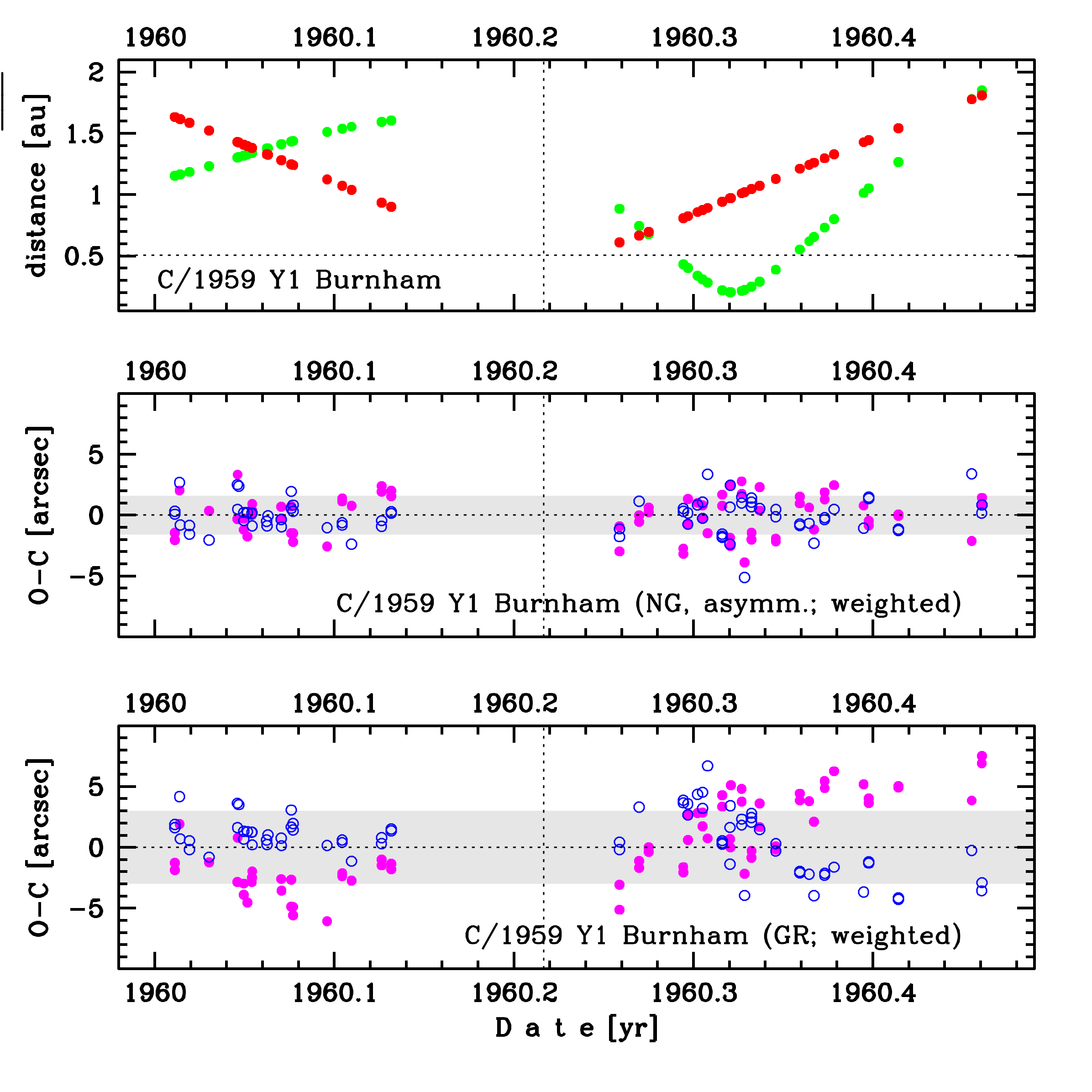
Upper panel: Time distribution of positional observations with corresponding heliocentric (red curve) and geocentric (green curve) distance at which they were taken. The horizontal dotted line shows the perihelion distance for a given comet whereas vertical dotted line — the moment of perihelion passage.
Lower panel (panels): O-C diagram for this(two) solution (solutions) given in this database, where residuals in right ascension are shown using magenta dots and in declination by blue open circles.
Lower panel (panels): O-C diagram for this(two) solution (solutions) given in this database, where residuals in right ascension are shown using magenta dots and in declination by blue open circles.
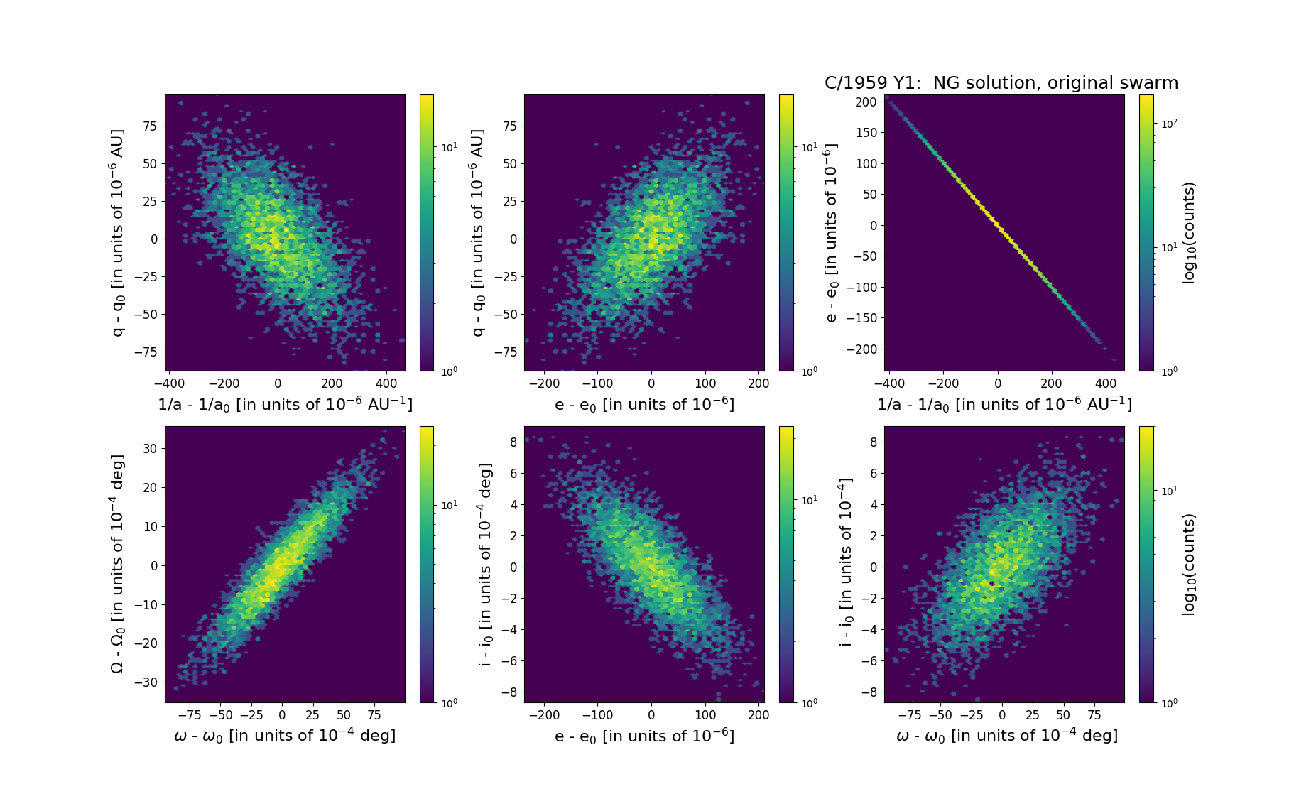
Six 2D-projections of the 6D space of original swarm including 5001 VCs. Each density map is given in logarithmic scale presented on the right in the individual panel.