C/2010 S1 LINEAR
more info
Comet C/2010 S1 was discovered on 21 September 2010 and next observed almost continuously by 4.8 yr in a range of heliocentric distances: 8.85 au – 5.900 au (perihelion) – 8.02 au. At the moment of discovery, it was two years and eight months before perihelion passage (see figure).
Comet had its closest approach to the Earth on 4 August 2013 (5.205 au, 2.5 months after perihelion).
NG orbit is possible to obtained using the full data arc; however uncertainties of NG parameters are notable, especially for A2 (see solutions ac and bc differing only in data weighting).
This Oort spike comet suffers a tiny planetary perturbations during its passage through the planetary system.
See also Królikowska and Dones 2023 and Królikowska and Dybczyński 2017.
| solution description | ||
|---|---|---|
| number of observations | 5260 | |
| data interval | 2010 09 21 – 2013 05 20 | |
| data arc selection | data generally limited to pre-perihelion (PRE) | |
| range of heliocentric distances | 8.85 au – 5.9au | |
| detectability of NG effects in the comet's motion | comet with determinable NG~orbit | |
| type of model of motion | GR - gravitational orbit | |
| data weighting | YES | |
| number of residuals | 10357 | |
| RMS [arcseconds] | 0.39 | |
| orbit quality class | 1a+ | |
| orbital elements (barycentric ecliptic J2000) | ||
|---|---|---|
| Epoch | 1706 06 07 | |
| perihelion date | 2013 05 19.85540364 | ± 0.00024014 |
| perihelion distance [au] | 5.90052484 | ± 0.00000152 |
| eccentricity | 0.99985137 | ± 0.00000124 |
| argument of perihelion [°] | 118.595814 | ± 0.000026 |
| ascending node [°] | 93.453968 | ± 0.000006 |
| inclination [°] | 125.320389 | ± 0.000002 |
| reciprocal semi-major axis [10-6 au-1] | 25.19 | ± 0.21 |
| file containing 5001 VCs swarm |
|---|
| 2010s1pa.bmi |
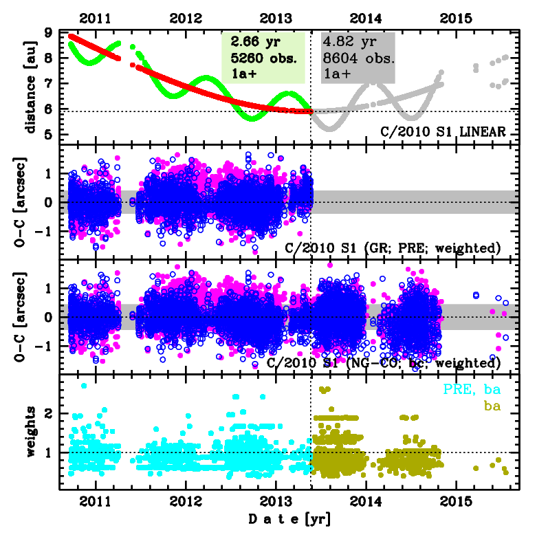
Upper panel: Time distribution of positional observations with corresponding heliocentric (red curve) and geocentric (green curve) distance at which they were taken. The horizontal dotted line shows the perihelion distance for a given comet whereas vertical dotted line — the moment of perihelion passage.
Middle panel(s): O-C diagram for a given solution (sometimes in comparison to another solution available in CODE), where residuals in right ascension are shown using magenta dots and in declination by blue open circles.
Lowest panel: Relative weights for a given data set(s).
Middle panel(s): O-C diagram for a given solution (sometimes in comparison to another solution available in CODE), where residuals in right ascension are shown using magenta dots and in declination by blue open circles.
Lowest panel: Relative weights for a given data set(s).
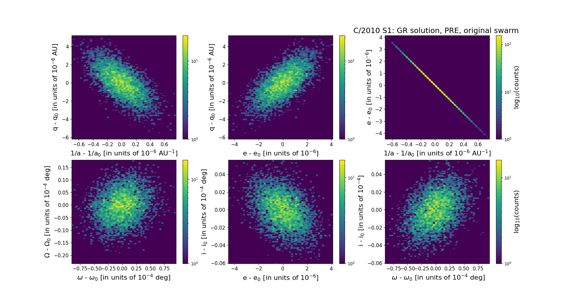
Six 2D-projections of the 6D space of original swarm including 5001 VCs. Each density map is given in logarithmic scale presented on the right in the individual panel.