C/2011 L2 McNaught
more info
Comet C/2011 L2 was discovered on 2 June 2011 by Robert H. McNaught (Siding Spring); that is about 5 months before its perihelion passage. The comet was observed until 28 January 2012.
Comet had its closest approach to the Earth on 27 July 2011 (1.500 au), almost 2 months after discovery and about 3 months before its perihelion passage.
Solutions given here are based on data spanning over 0.657 yr in a range of heliocentric distances: 2.66 au – 1.943 au (perihelion) – 2.22 au. The non-gravitational solution was chosen as preferred orbit; however, uncertainties of NG parameters are large.
This Oort spike comet suffers small planetary perturbations during its passage through the planetary system; these perturbations lead to a more tight future orbit (see future barycentric orbits).
See also Królikowska 2020.
| solution description | ||
|---|---|---|
| number of observations | 59 | |
| data interval | 2011 06 02 – 2012 01 28 | |
| data type | perihelion within the observation arc (FULL) | |
| data arc selection | entire data set (STD) | |
| range of heliocentric distances | 2.66 au – 1.94 au (perihelion) – 2.22 au | |
| type of model of motion | NS - non-gravitational orbits for standard g(r) | |
| data weighting | NO | |
| number of residuals | 107 | |
| RMS [arcseconds] | 0.41 | |
| orbit quality class | 1b | |
| orbital elements (barycentric ecliptic J2000) | ||
|---|---|---|
| Epoch | 2313 07 02 | |
| perihelion date | 2011 11 01.44673645 | ± 0.00279038 |
| perihelion distance [au] | 1.94002998 | ± 0.00001778 |
| eccentricity | 0.99968336 | ± 0.00003570 |
| argument of perihelion [°] | 256.916400 | ± 0.001541 |
| ascending node [°] | 131.392710 | ± 0.000433 |
| inclination [°] | 104.367542 | ± 0.000242 |
| reciprocal semi-major axis [10-6 au-1] | 163.21 | ± 18.40 |
| file containing 5001 VCs swarm |
|---|
| 2011l2n1.bpl |
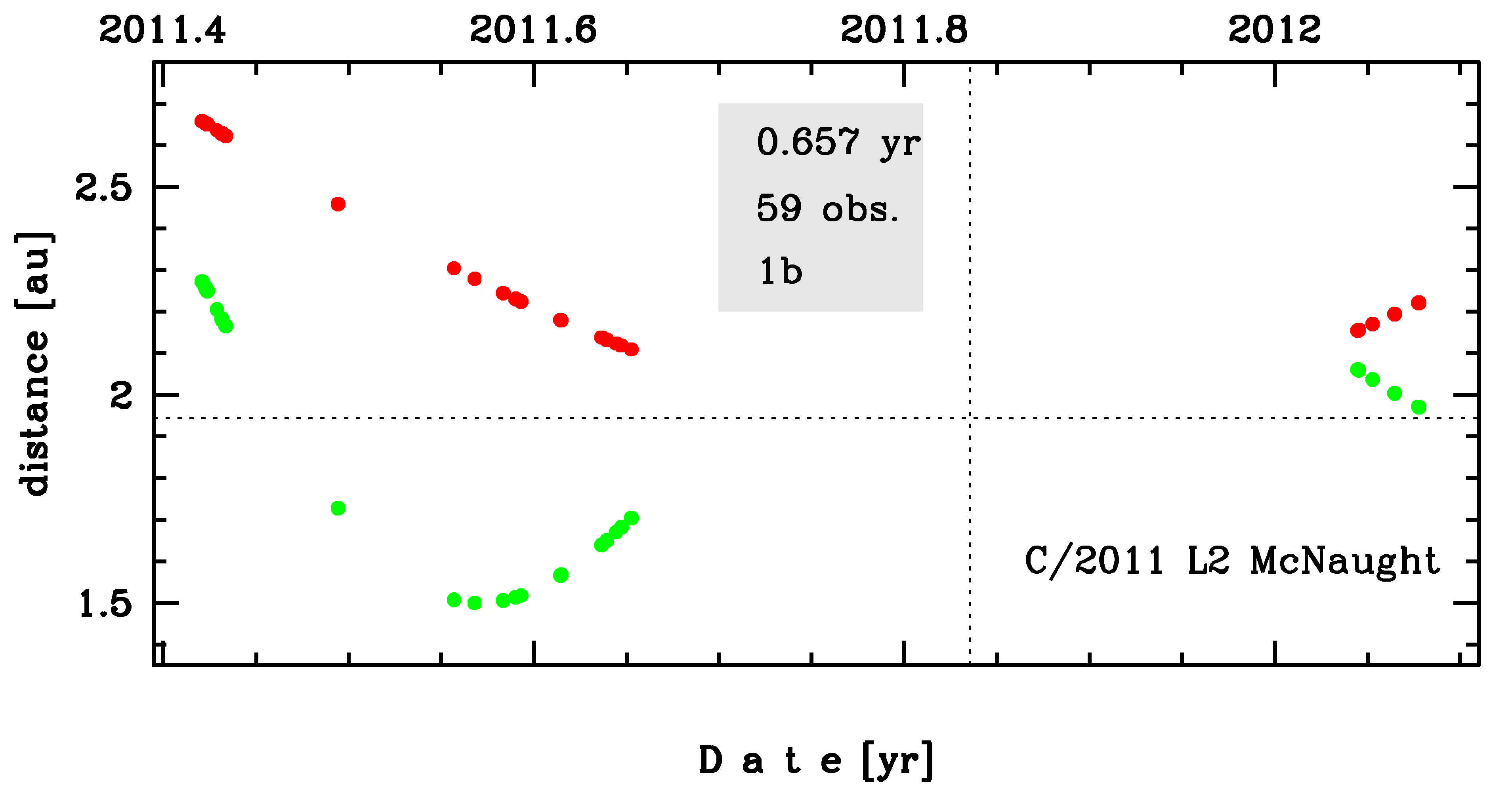
Time distribution of positional observations with corresponding heliocentric (red curve) and geocentric (green curve) distance at which they were taken. The horizontal dotted line shows the perihelion distance for a given comet whereas vertical dotted line — the moment of perihelion passage.
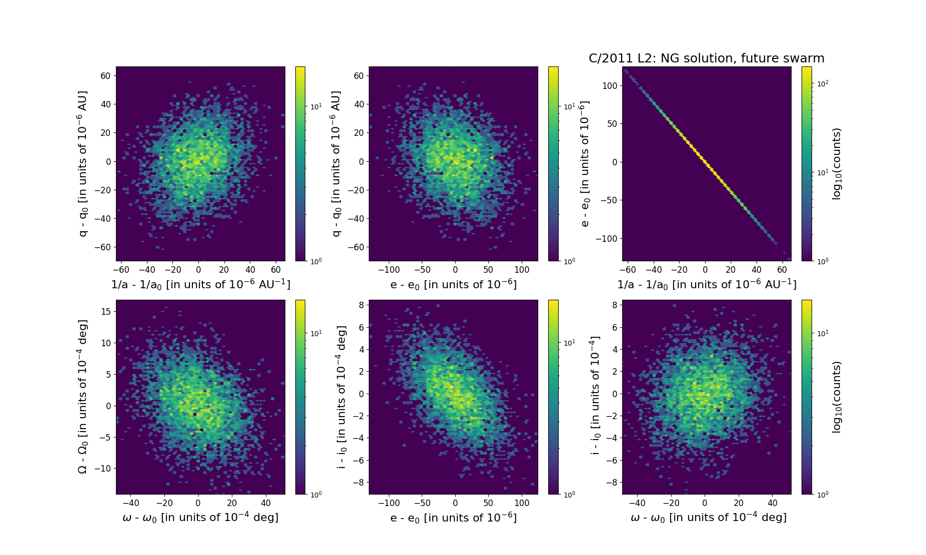
Six 2D-projections of the 6D space of future swarm including 5001 VCs. Each density map is given in logarithmic scale presented on the right in the individual panel.