C/1902 X1 Giacobini
more info
Comet C/1902 X1 was discovered on 2 December 1902 by Michel Giacobini (Nice Observatory, France), that is almost four months before perihelion passage, and it was last seen on 27 June 1903 [Kronk, Cometography: Volume 3].
This comet made its closest approach to the Earth on 18 January 1903 (1.91 au), that is about seven weeks after its discovery.
Solution given here is based on data spanning over 0.567 yr in a narrow range of heliocentric distances from 3.00 au through perihelion (2.77 au) to 2.94 au.
This Oort spike comet suffers moderate planetary perturbations during its passage through the planetary system that lead to escape the comet from the planetary zone on a hyperbolic orbit (see future barycentric orbit)
More details in Królikowska et al. 2014.
| solution description | ||
|---|---|---|
| number of observations | 735 | |
| data interval | 1902 12 02 – 1903 06 27 | |
| data type | perihelion within the observation arc (FULL) | |
| data arc selection | entire data set (STD) | |
| range of heliocentric distances | 3 au – 2.77 au (perihelion) – 2.94 au | |
| detectability of NG effects in the comet's motion | NG effects not determinable | |
| type of model of motion | GR - gravitational orbit | |
| data weighting | YES | |
| number of residuals | 1307 | |
| RMS [arcseconds] | 1.66 | |
| orbit quality class | 1b | |
| orbital elements (barycentric ecliptic J2000) | ||
|---|---|---|
| Epoch | 1601 01 28 | |
| perihelion date | 1903 03 24.05943308 | ± 0.00249302 |
| perihelion distance [au] | 2.77648897 | ± 0.00001348 |
| eccentricity | 0.99979445 | ± 0.00002012 |
| argument of perihelion [°] | 5.819304 | ± 0.000769 |
| ascending node [°] | 118.884571 | ± 0.000087 |
| inclination [°] | 43.892926 | ± 0.000261 |
| reciprocal semi-major axis [10-6 au-1] | 74.03 | ± 7.25 |
| file containing 5001 VCs swarm |
|---|
| 1902x1a5.bmi |
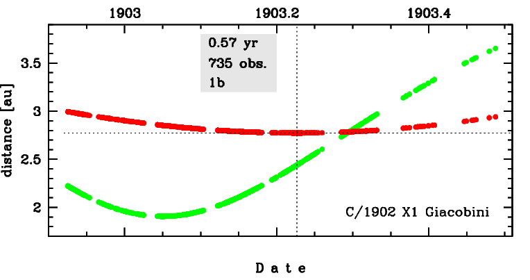
Time distribution of positional observations with corresponding heliocentric (red curve) and geocentric (green curve) distance at which they were taken. The horizontal dotted line shows the perihelion distance for a given comet whereas vertical dotted line — the moment of perihelion passage.
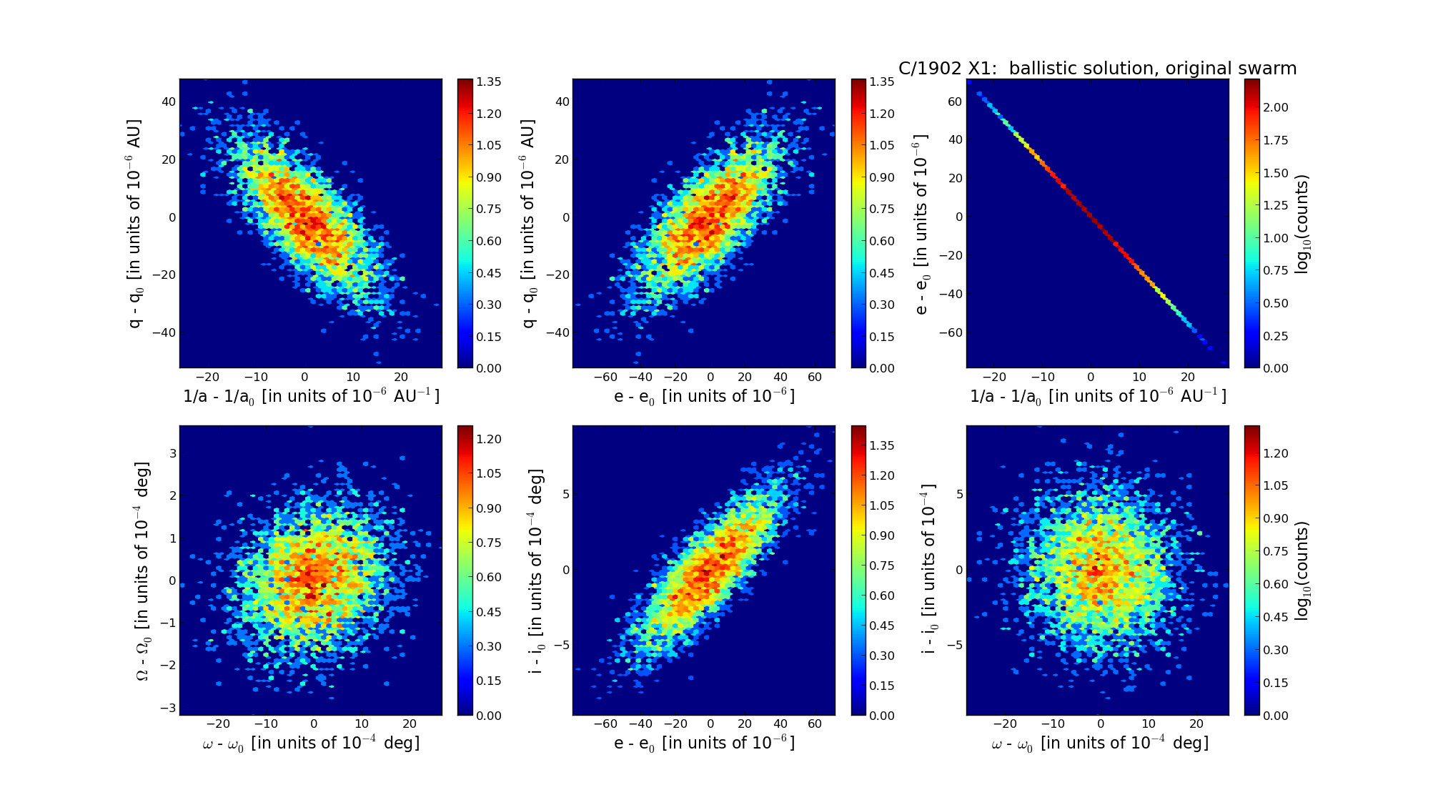
Six 2D-projections of the 6D space of original swarm including 5001 VCs. Each density map is given in logarithmic scale presented on the right in the individual panel.