C/2017 B3 LINEAR
more info
Comet C/2017 B3 was discovered on 26 January 2017 with the LINEAR survey, , that is about two years before its perihelion passage. Some prediscovery images of this comet were found: taken on 1 and 10 of Aprilnbsp;2016 by the Pan-STARRS 1 telescope (Haleakala).
Comet had its closest approach to the Earth on 19nbsp;Augustnbsp;2019 (3.480nbsp;au), about a 6.5nbsp;months after its perihelion passage.
Preferred NGnbsp;solution given here is based on data arc spanning over 5.83nbsp;yr in a range of heliocentric distances: 9.16 au – 3.92 au (perihelion) – 9.15 au.
This comet suffers small planetary perturbations during its passage through the planetary system; this is a long-period comet with original and future semimajor axes of about 3,300 au, and 2,100 au, respectively.
| solution description | ||
|---|---|---|
| number of observations | 1587 | |
| data interval | 2016 03 04 – 2022 01 01 | |
| data type | perihelion within the observation arc (FULL) | |
| data arc selection | entire data set (STD) | |
| range of heliocentric distances | 9.16 au – 3.92 au (perihelion) – 9.15 au | |
| type of model of motion | NC - non-gravitational orbits for symmetric CO-g(r)-like function | |
| data weighting | YES | |
| number of residuals | 3107 | |
| RMS [arcseconds] | 0.34 | |
| orbit quality class | 1a+ | |
| orbital elements (barycentric ecliptic J2000) | ||
|---|---|---|
| Epoch | 1712 03 27 | |
| perihelion date | 2019 02 02.59323696 | ± 0.00041025 |
| perihelion distance [au] | 3.92467200 | ± 0.00000445 |
| eccentricity | 0.99882347 | ± 0.00000264 |
| argument of perihelion [°] | 284.667858 | ± 0.000092 |
| ascending node [°] | 2.228655 | ± 0.000007 |
| inclination [°] | 54.290403 | ± 0.000008 |
| reciprocal semi-major axis [10-6 au-1] | 299.78 | ± 0.67 |
| file containing 5001 VCs swarm |
|---|
| 2017b3c6.bmi |

Upper panel: Time distribution of positional observations with corresponding heliocentric (red curve) and geocentric (green curve) distance at which they were taken. The horizontal dotted line shows the perihelion distance for a given comet whereas vertical dotted line — the moment of perihelion passage.
Middle panel(s): O-C diagram for a given solution (sometimes in comparison to another solution available in CODE), where residuals in right ascension are shown using magenta dots and in declination by blue open circles.
Lowest panel: Relative weights for a given data set(s).
Middle panel(s): O-C diagram for a given solution (sometimes in comparison to another solution available in CODE), where residuals in right ascension are shown using magenta dots and in declination by blue open circles.
Lowest panel: Relative weights for a given data set(s).
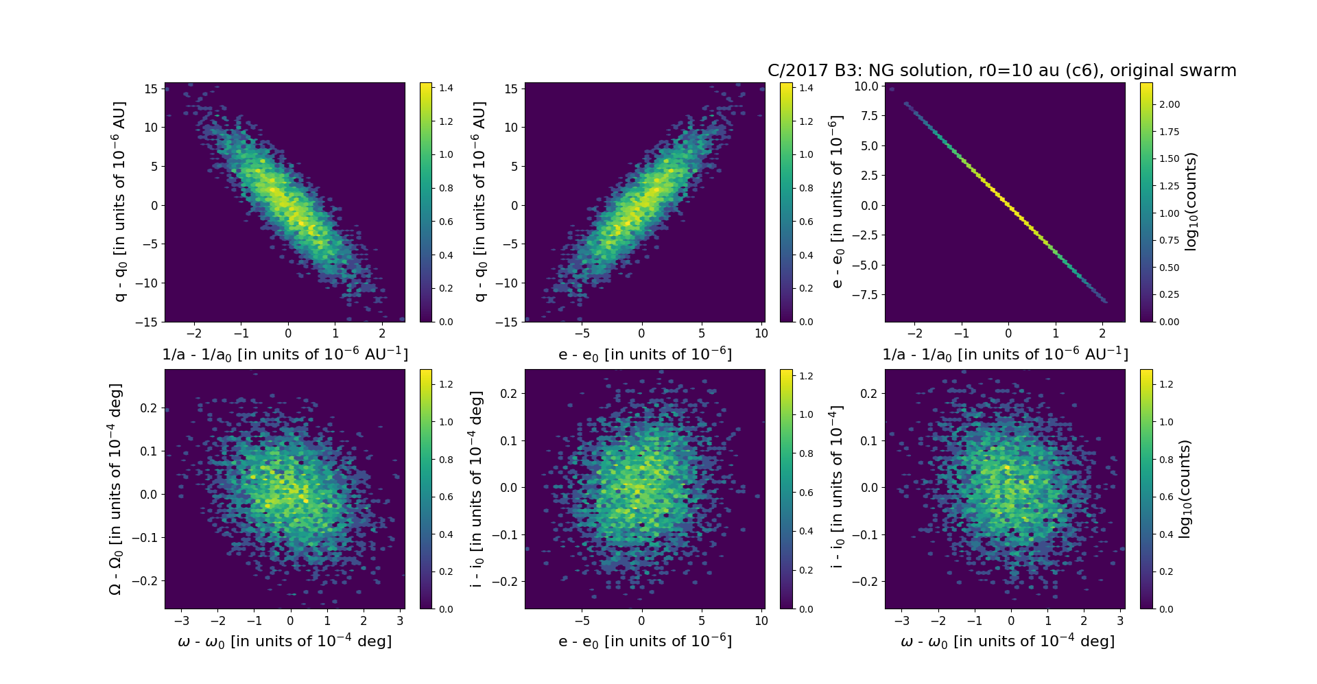
Six 2D-projections of the 6D space of original swarm including 5001 VCs. Each density map is given in logarithmic scale presented on the right in the individual panel.