C/2015 X7 ATLAS
more info
Comet C/2015 X7 was discovered on 12 December 2015 by Asteroid Terrestrial-impact Last Alert System (ATLAS) Team, that is about 7.5 months before its perihelion passage. Some prediscovery images of this comet were found: taken on 28 January 2015 by Pan-STARRS 1, Haleakala. This comet was observed until 16 June 2017.
Comet had its closest approach to the Earth on 8 February 2017 (5.909 au); about 6 months after its perihelion passage.
Solutions given here are based on data spanning over 2.38 yr in a range of heliocentric distances: 5.95 au – 3.685 au (perihelion) – 4.64 au.
This Oort spike comet suffers small planetary perturbations during its passage through the planetary system that lead to a more tight future orbit with a semimajor axis of about 5,000 au (see future barycentric orbits).
| solution description | ||
|---|---|---|
| number of observations | 628 | |
| data interval | 2015 01 28 – 2017 06 16 | |
| data type | perihelion within the observation arc (FULL) | |
| data arc selection | entire data set (STD) | |
| range of heliocentric distances | 5.95 au – 3.69 au (perihelion) – 4.64 au | |
| type of model of motion | NC - non-gravitational orbits for symmetric CO-g(r)-like function | |
| data weighting | YES | |
| number of residuals | 1244 | |
| RMS [arcseconds] | 0.43 | |
| orbit quality class | 1a+ | |
| orbital elements (barycentric ecliptic J2000) | ||
|---|---|---|
| Epoch | 2321 10 21 | |
| perihelion date | 2016 07 30.28304629 | ± 0.00139261 |
| perihelion distance [au] | 3.67857133 | ± 0.00001049 |
| eccentricity | 0.99926420 | ± 0.00000905 |
| argument of perihelion [°] | 348.380323 | ± 0.000278 |
| ascending node [°] | 139.787845 | ± 0.000035 |
| inclination [°] | 57.592181 | ± 0.000032 |
| reciprocal semi-major axis [10-6 au-1] | 200.02 | ± 2.46 |
| file containing 5001 VCs swarm |
|---|
| 2015x7c5.bpl |
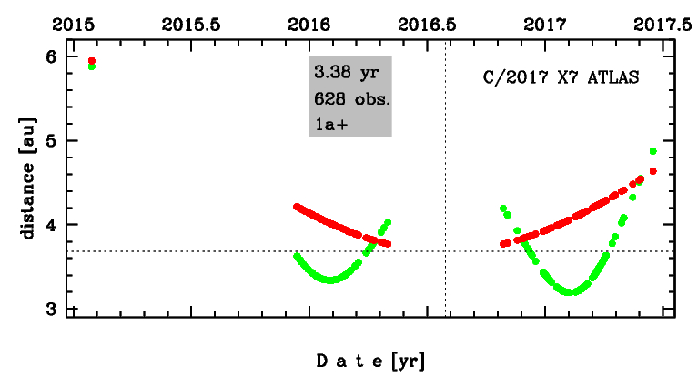
Time distribution of positional observations with corresponding heliocentric (red curve) and geocentric (green curve) distance at which they were taken. The horizontal dotted line shows the perihelion distance for a given comet whereas vertical dotted line — the moment of perihelion passage.
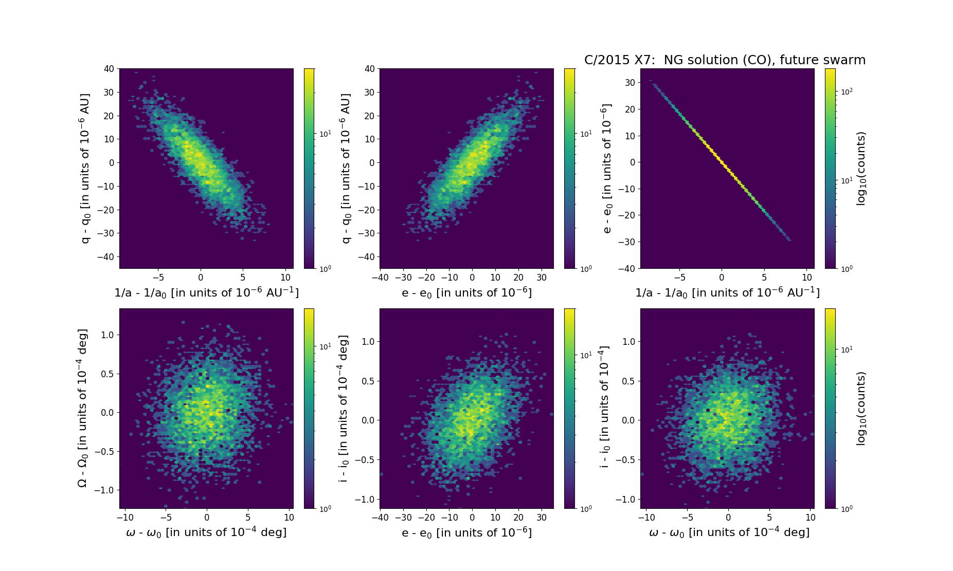
Six 2D-projections of the 6D space of future swarm including 5001 VCs. Each density map is given in logarithmic scale presented on the right in the individual panel.